“Old-school” PyFVTool: the heat equation in a 1D Cartesian system

This particular Notebook demonstrates the “old-school” expert approach to setting up the finite-volume solution to the heat equation using PyFVTool. The discretized terms of the matrix equation are explicitly evaluated and cast into the final sparse matrix equation which is then solved numerically with pf.solveMatrixPDE().

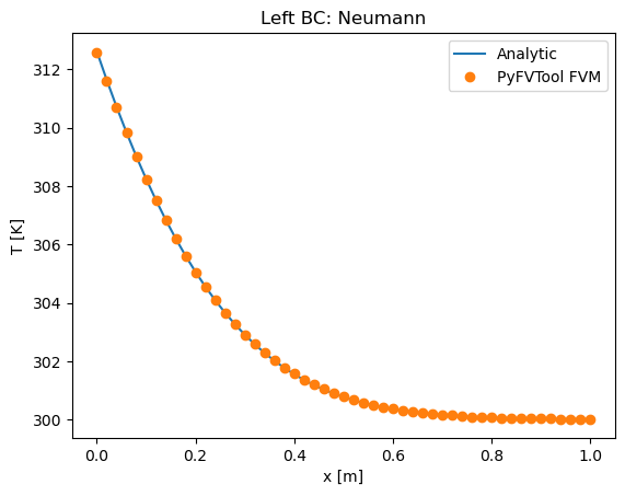
This example illustrates the inner workings of the finite-volume method. It is functionally and numerically identical to cartesian1D_heat_equation_neumann.ipynb. We compare the FVM solution by PyFVTool to the analytic solutions.

import numpy as np
from scipy.special import erf
import matplotlib.pyplot as plt
import pyfvtool as pf

# Spoiler alert!

def T_analytic_dirichlet(x,t, alfa, T0, Ts):
    return (T0-Ts)*erf(x/np.sqrt(4*alfa*t))+Ts

def T_analytic_neumann(x,t, alfa, T0, k, qs):
    return T0 + qs/k*np.sqrt(4*alfa*t/np.pi)*np.exp(-x**2/(4*alfa*t))\
              - qs/k*x*(1-erf(x/np.sqrt(4*alfa*t)))

# Parameters
L = 1.0 # [m] domain length
k = 20.0 # 0.6 for water, 0.025 for air W/m/K
rho = 8000.0 # kg/m^3
c = 500.0 # J/kg/K (4200 for water, 1000 for air)
alfa = k/(rho*c) # heat diffusion
T0 = 300.0 # [K]
Ts = 350.0 # [K]
qs = 1000 # [W/m^2]
t_sim = L**2/(20*alfa) # [s]
time_steps = 50
dt = t_sim/time_steps #
Nx = 50 # number of cells

m = pf.Grid1D(Nx, L)

# Boundary condition
left_bc = "Neumann"

BC = pf.BoundaryConditions(m)
if left_bc == "Dirichlet":
    BC.left.a[:] = 0.0
    BC.left.b[:] = 1.0
    BC.left.c[:] = Ts
    T_analytic = lambda x,t: T_analytic_dirichlet(x, t, alfa, T0, Ts)
else:
    BC.left.a[:] = k
    BC.left.b[:] = 0.0
    BC.left.c[:] = -qs
    T_analytic = lambda x,t: T_analytic_neumann(x, t, alfa, T0, k, qs)

# Initial condition
T_init = pf.CellVariable(m, T0, BC) # initial condition

# physical parameters
alfa_cell = pf.CellVariable(m, alfa, pf.BoundaryConditions(m))
alfa_face = pf.harmonicMean(alfa_cell)

M_diff = pf.diffusionTerm(alfa_face)
[M_bc, RHS_bc] = pf.boundaryConditionsTerm(BC)

t=0
while t<t_sim:
    t +=dt
    [M_trans, RHS_trans] = pf.transientTerm(T_init, dt, 1.0)
    T_val = pf.solveMatrixPDE(m, M_bc+M_trans-M_diff, RHS_bc+RHS_trans)
    T_init.update_value(T_val)

x = m.facecenters.x
T_face = pf.linearMean(T_val)
T_num = T_face.xvalue
T_an = T_analytic(x, t_sim)

plt.figure(1)
plt.clf()
plt.title('Left BC: '+left_bc)
plt.plot(x, T_an, x, T_num, 'o')
plt.legend({'Analytic', 'PyFVTool FVM'})
plt.xlabel('x [m]')
plt.ylabel('T [K]')
plt.show()

er = np.sum(np.abs(T_num-T_an)/T_an)/Nx
print(er)

4.1994295875793644e-05