1D wave equation

Written by Ali A. Eftekhari

• Last checked: June 2021

• Ported to Python by Gavin M. Weir, June 2023

• Update by M. H. V. Werts, October 2025

PDE and boundary conditions

The homogeneous wave equation reads

\[\frac{\partial^2 c}{\partial t^2} = u^2 \frac{\partial^2 c}{\partial x^2},\]

where \(c\) is the independent variable (displacement, concentration, temperature, etc), \(u\) is the characteristic velocity.

The inhomogeneous wave equation with initial conditions on the value and derivative of the concentration takes the form

\[\frac{\partial^2 c\left(x,t\right)}{\partial t^2} - u^2 \frac{\partial^2 c\left(x,t\right)}{\partial x^2} = s\left(x,t\right)\]

\[c\left(x, 0\right) = f\left(x\right)\]

\[\frac{\partial c}{\partial t}\left(x, 0\right) = g\left(x\right)\]

import pyfvtool as pf
import numpy as np

# for animation and visualization
import matplotlib.pyplot as plt
from matplotlib.animation import FuncAnimation

def c(x):
    return x*x

def dc(x):
    return 2.0*x

Lx = float(1.0)   # length of domain
Nx = int(200)     # number of cells in domain
dx = Lx/Nx        # step-size in uniform 1d grid
m = pf.Grid1D(Nx, Lx) # 1D domain

x_face=m.facecenters.x   # face positions
x_cell=m.cellcenters.x   # node positions

# initial value on grid
u0 = np.abs(np.sin(x_cell/Lx*10*np.pi))

# Velocity on grid nodes (cell centers)
u = pf.CellVariable(m, u0);

# Boundary conditions
u.BCs.left.periodic = True
u.BCs.right.periodic = True

# Initialize the face concenrtation values and their derivatives at the faces
c_face = pf.FaceVariable(m, 0.0)     # concentration values
c_face.xvalue = c(x_face)

# concentration derivative
dc_cell = pf.CellVariable(m, dc(x_cell))

dt = 0.1  # time-step for calculations

ui = [u.copy()] # store initial condition
for ii in range(2000):
    # Solve the PDE, single time step
    pf.solvePDE(u, [ pf.transientTerm(u, dt, 1.0),
                     pf.convectionUpwindTerm(c_face),
                    -pf.linearSourceTerm(dc_cell)])
    # Store solution at next index
    ui.append(u.copy())    # It is essential to COPY the CellVariable
                           # if the current values need to be conserved for the future.
                           # Each call to solvePDE() replaces the values in the original
                           # CellVariable.

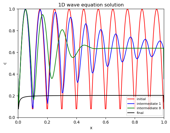
# Plotting and visualization of the 1D wave equation solution

hfig1, ax1 = plt.subplots()

xx, uu = ui[0].plotprofile()
ax1.plot(xx, uu, 'r-', label='initial')

xx, uu = ui[1].plotprofile()
ax1.plot(xx, uu, 'b-', label='intermediate 1')

xx, uu = ui[8].plotprofile()
ax1.plot(xx, uu, 'g-', label='intermediate 8')

xx, uu = ui[-1].plotprofile()
ax1.plot(xx, uu, 'k-', label='final')

ax1.set_xlim((0, Lx))
ax1.set_ylim((0.0, 1.0))

ax1.set_xlabel('x')
ax1.set_ylabel('c')
ax1.set_title('1D wave equation solution')
ax1.legend(fontsize=8);

# ========= # # ANIMATION NEEDS TO BE ADAPTED FOR INTERACTIVE NOTEBOOK # create a figure to handle the solution animation # pre-generate the handles to the axes and the line hfig2 = plt.figure() ax2 = plt.axes(xlim=(0, Lx), ylim=(0.0, 1.0)) line, = ax2.plot([], [], 'k-', lw=3, label='Numerical solution') ax2.set_xlabel('x') ax2.set_ylabel('c') ax2.set_title('1D wave equation solution') ax2.legend(fontsize=8) def init(): line.set_data([], []) return line, def animate(ii): # x, y = get_CellVariable_profile1D(ui[ii]) global ui line.set_data(*get_CellVariable_profile1D(ui[ii])) return line, anim = FuncAnimation(hfig2, animate, init_func=init, frames=400, interval=20, blit=True)