Using Intel oneMKL PARDISO as an external sparse direct solver for PyFVTool
MW 250721
This is an example of how to use an external sparse solver via a PyFVTool interface.
An external solver can be supplied as an optional argument to pyfvtool.solvePDE(), e.g.
pf.solvePDE(phi, eqnterms,
            externalsolver = solveur)
where solveur is a function that will be called instead of scipy.sparse.linalg.spsolve(A, b). It should provide the same interface as the original spsolve.
In this example, we use pyfvtool.solvers.oneMKL_pardiso.spsolve_oneMKL_pardiso(A, b).
PyFVTool MKL PARDISO interface
PyFVTool includes a minimal interface to the Intel oneMKL PARDISO solver
Beyond numpy, scipy and matplotlib, it requires that the Intel oneMKL runtime (package mkl) be installed in the PyFVTool environment. On Windows, this may already be the case, since NumPy already depends on it, but we found that it needs to be installed explicitly on our Linux system:
conda install mkl
Test drive the solver
[1]:
import sys
import numpy as np
import scipy as sp
from scipy import sparse
import matplotlib.pyplot as plt
[2]:
from time import time
import pyfvtool as pf
[3]:
from pyfvtool.solvers.oneMKL_pardiso import spsolve as spsolve_oneMKL_pardiso

# additional import to get MKL version printed
from pyfvtool.solvers.oneMKL_pardiso import oneMKL_pardiso_solver_instance
[4]:
print('Python', sys.version)
print('NumPy version          : ', np.__version__)
print('SciPy version          : ', sp.__version__)
print('oneMKL runtime version : ', oneMKL_pardiso_solver_instance.get_MKL_version_string())
print('PyFVTool version       : ', pf.__version__)
Python 3.12.9 | packaged by conda-forge | (main, Mar  4 2025, 22:37:18) [MSC v.1943 64 bit (AMD64)]
NumPy version          :  2.3.0
SciPy version          :  1.15.2
oneMKL runtime version :  2025.0.1
PyFVTool version       :  0.4.2
[5]:
A = sparse.rand(10, 10, density=0.5, format='csr')
[6]:
b = np.random.rand(10)
[7]:
x = spsolve_oneMKL_pardiso(A, b)
[8]:
x
[8]:
array([ 4.90190165,  0.7385448 , -2.45810562,  1.8050738 ,  1.65217373,
        0.98397367,  1.01222876, -0.27855745, -4.20957481, -3.05200821])
PyFVTool finite-volume (from cylindrical2D_convection notebook)
Utility functions
[9]:
# visualization routine (imshow-based)
def phi_visualize():
    print(f't = {t:.1f} s')
    # avoid ghost cells
    plt.imshow(phi.value, origin = 'lower',
               extent = [zz[0], zz[-1], rr[0]*rzoom, rr[-1]*rzoom])
[10]:
# calculate simple finite-volume integral over r
def integral_dr(phi0):
    v = phi0.cellvolume
    c = phi0.value
    return (v*c).sum(axis=0)
FVM settings
[11]:
Lr = 7.5e-05 # [m] radius of cylinder
Lz = 0.3 # [m] length of cylinder
umax = 2*9.4314e-3 # [m s^-1] max flow velocity = 2 time average flow velocity
[12]:
# regular grid parameters
Nr = 40
Nz = 500
[13]:
# initial condition parameters (cell indices)
loadix0 = 20
loadix1 = 40
[14]:
# timestep parameters
deltat = 0.01 # [s] per time step
[15]:
# visualization parameters
rzoom = 1000
2D cylindrical mesh
[16]:
msh = pf.CylindricalGrid2D(Nr, Nz, Lr, Lz)
Set up Poiseuille flow velocity field
[17]:
rr = msh.cellcenters.r
zz = msh.facecenters.z
[18]:
uu = umax*(1 - (rr**2)/(Lr**2)) # does not depend on zz
[19]:
u = pf.FaceVariable(msh, 1.0)
[20]:
u.rvalue[:] = 0
u.zvalue[:] = uu[:, np.newaxis]
Solution variable
[21]:
bc = pf.BoundaryConditions(msh)
[22]:
phi = pf.CellVariable(msh, 0.0 , bc)
Initial condition
[23]:
t=0.
[24]:
# initial condition
for i in range(loadix0, loadix1):
    phi.value[:, i] = 1.0
[25]:
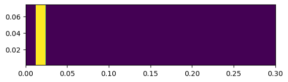
phi_visualize()
t = 0.0 s
[26]:
initInt = phi.domainIntegral()
# print(initInt)
[27]:
phiprofs = []
phiprofs.append((t, integral_dr(phi)))
Solve the convection PDE with time-stepping
[28]:
exect0 = time()
[29]:
# The convection term only needs to be constructed once, since it
# will be constant during all time steps.
# convectionterm = pf.convectionTerm(u) # really ugly results?
convectionterm = pf.convectionUpwindTerm(u) # numerical diffusion

def step_solver(Nstp):
    global t

    for i in range(Nstp):
        # Transient term needs to be re-evaluated at each time step
        transientterm = pf.transientTerm(phi, deltat, 1.0)
        eqnterms = [transientterm,
                    convectionterm]
        # solve the PDE using oneMKL PARDISO as the external solver,
        #    via `spsolve_oneMKL_pardiso`
        pf.solvePDE(phi, eqnterms,
                    externalsolver = spsolve_oneMKL_pardiso)
        t += deltat
[30]:
step_solver(200)
phiprofs.append((t, integral_dr(phi)))
[31]:
# print(t, initInt, pf.domainInt(phi))
# test conservation of mass
assert np.isclose(initInt, phi.domainIntegral())
[32]:
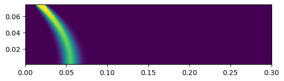
phi_visualize()
t = 2.0 s
[33]:
step_solver(300)
phiprofs.append((t, integral_dr(phi)))
[34]:
step_solver(500)
phiprofs.append((t, integral_dr(phi)))
[35]:
print(t, initInt, phi.domainIntegral())
9.999999999999831 2.1205750411731096e-10 2.1205750411729896e-10
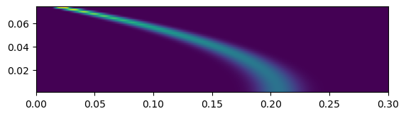
[36]:
phi_visualize()
t = 10.0 s
[37]:
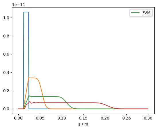
for ix, (tprof, phiprof) in enumerate(phiprofs):
    if ix == 2:
        lbl1 = 'FVM'
    else:
        lbl1 = None
    plt.plot(phi.domain.cellcenters.z, phiprof,
             label=lbl1)
plt.xlabel('z / m')
plt.legend();
[38]:
exect1 = time()
[39]:
print('Elapsed time ', exect1 - exect0, 's')
Elapsed time 6.2673749923706055 s
[ ]: