Poisson equation example

• Written by Ali A. Eftekhari (last update 2021)

• Ported to Python and full rewrite by Gavin M. Weir June, 2023.

The generalized form of the equations solved in this package looks like,

\[\alpha \frac{\partial \varphi}{\partial t} + \nabla\cdot\left(\vec{u}\varphi\right) + \nabla\cdot\left(-D\nabla\varphi\right) + \beta \varphi = \gamma\]

with boundary condition,

\[a\nabla\varphi\cdot \vec{e} + b\varphi = c\]

.

The inhomogeneous Poisson equation

\[\nabla^2 \varphi + s\left(\vec{x}\right) = 0\]

can be generalized to a simple 1D case,

\[\begin{split}\begin{align} \frac{\partial^2 \varphi}{\partial ^2 x} + s\left(x\right) &= 0 \\ \varphi\left(x_L\right) &= 0 \\ \frac{\partial \varphi}{\partial x}|_{x_R} &= 0 \end{align}\end{split}\]

The corresponding equation in our form has

\[\begin{split}\begin{align} D = 1.0, \vec{u} &= \vec{0} \\ \alpha = 0, \beta = 0, \gamma &= s \\ a_L = 0, b_L = 1, c_L &= 0 \\ a_R = 1, b_R = 0, c_R &= 0 \\ \end{align}\end{split}\]

see this link http://scicomp.stackexchange.com/questions/8577/peculiar-error-when-solving-the-poisson-equation-on-a-non-uniform-mesh-1d-only

Strange behavior when change the number of grids from even to odd Wrong results does not always mean that the code has bugs.

Wrong use of the code can also give you wrong results.

import numpy as np
import matplotlib.pyplot as plt

# explicit imports as an alternative to `import pyfvtool as pf`
from pyfvtool import Grid1D
from pyfvtool import cellLocations, CellVariable
from pyfvtool import faceLocations, FaceVariable
from pyfvtool import BoundaryConditions
from pyfvtool import diffusionTerm
from pyfvtool import constantSourceTerm
from pyfvtool import boundaryConditionsTerm
from pyfvtool import solvePDE
from pyfvtool import visualizeCells

# Define the domain and create a mesh structure
L = 20      # domain length
# Nx = 10000  # number of cells (original)
Nx = 100000  # number of cells (test)
m = Grid1D(Nx, L)

# Solution variable
c = CellVariable(m, 0.0)

# Boundary Conditions

# Left boundary
c.BCs.left.a, c.BCs.left.b, c.BCs.left.c = 0.0, 1.0, 0.0

# Right boundary (Neumann zero-flux is the default in this package)
c.BCs.right.a, c.BCs.right.b, c.BCs.right.c = 1.0, 0.0, 0.0

# define the transfer coeffs
D_val = 1.0
D = FaceVariable(m, D_val)

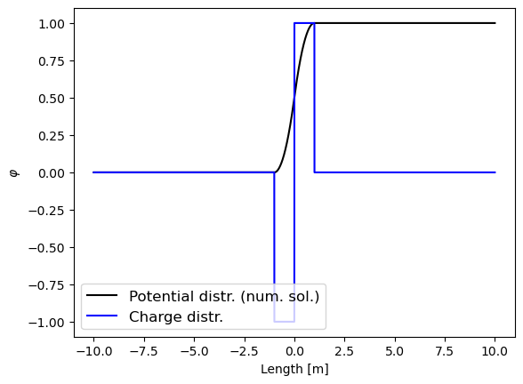
# define source term
def rho(x):
    return -1.0*((x>=-1.0)*(x<=0))+(x>0)*(x<=1)

x = m.cellcenters.x-0.5*L # shift the domain to [-10,10]

c = solvePDE(c, [-constantSourceTerm(CellVariable(m, rho(x))),
                  diffusionTerm(D)])

# visualization
plt.figure()
plt.plot(x, c.value, 'k-', label='Potential distr. (num. sol.)')
plt.plot(x, rho(x), 'b-', label='Charge distr.')
plt.xlabel('Length [m]')
plt.ylabel(r'$\varphi$')
plt.legend(fontsize=12, loc='best');