Heat transfer with time-variant boundary conditions

Heat transfer example based on a Julia example

see: https://docs.sciml.ai/MethodOfLines/stable/tutorials/heat/

import numpy as np
import matplotlib.pyplot as plt
import pyfvtool as pf

def T_analytic(x,t):
    return np.exp(-t)*np.cos(x)

# Parameters
L = 1.0 # domain length
alfa = 1.0 # heat diffusion
qs = 1000.0 # [W/m^2]
t_sim = L**2/(20*alfa) # [s]
time_steps = 50
dt = t_sim/time_steps #
Nx = 20 # number of cells

m = pf.Grid1D(Nx, L)

# Initial condition
T0 = np.cos(m.cellcenters.x) # cosine temperature profile, amplitude = 1.0 K
T = pf.CellVariable(m, T0) # initial condition

# Boundary conditions
T.BCs.left.a = 0.0
T.BCs.left.b = 1.0
T.BCs.right.a = 0.0
T.BCs.right.b = 1.0

# physical parameters
alfa_cell = pf.CellVariable(m, alfa)
alfa_face = pf.harmonicMean(alfa_cell)

M_diff = pf.diffusionTerm(alfa_face)

t=0
while t<t_sim:
    t +=dt
    T.BCs.left.c = np.exp(-t)
    T.BCs.right.c = np.exp(-t)*np.cos(L)
    pf.solvePDE(T, [ pf.transientTerm(T, dt, 1.0),
                    -pf.diffusionTerm(alfa_face)])

x = m.facecenters.x
T_face = pf.linearMean(T)
T_num = T_face.xvalue
T_an = T_analytic(x, t_sim)

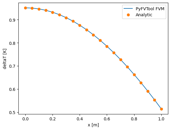
plt.figure(1)
plt.clf()
plt.plot(x, T_an, x, T_num, 'o')
plt.legend({'Analytic', 'PyFVTool FVM'})
plt.xlabel('x [m]')
plt.ylabel('deltaT [K]')
plt.show()

er = np.sum(np.abs(T_num-T_an)/T_an)/Nx
print(er)

0.00014085141590735798

assert er<0.0005